Purpose

The purpose of this notebook is to create a Python class that implements the logistic regression algorithm from only numpy.

Background

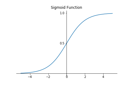
Logistic regression is an algorithm that is commonly used for binary classificaiton problems. It does this by predicting a probability and then using a threshold to determine which class to predict. Although the algorithm can be used for multi-class prediction problems, only binary classification is considered in this notebook. The following (sigmoid) function transforms the linear model into the range [0,1]:

$$\sigma(x) = \frac{1}{1+e^{-x}}$$

Visualising this function produces the following graph:

Cost Function

The cost function used for linear regression does not work for logistic regression. This is because the sigmoid function causes many local minimums, meaning that finding optimal weights to minimise the cost function proves difficult. Therefore, the cross-entropy loss function is used to produce the following cost function:

$$ \begin{align} J(\theta) = &- \frac{1}{m} \sum^m_{i=1} [y^{(i)} \log(h_{\theta}(x^{(i)})) + (1 - y^{(i)}) \log(1 - h_{\theta}(x^{(i)}))] \\ = &- \frac{1}{m} (y^T \log(h) + (1 - y)^T \log(1-h)) \end{align} $$

Where $ h = X \theta$.

Gradient Descent

As the logistic regression does not have a closed form solution, like the basic linear regression, gradient descent is used to find the optimal weights that minimise the cost function. The partial derivative of the cost function with respect to each weight is as follows:

$$ \begin{align} \frac{\partial L}{\partial w_j} = [\sigma(X \theta) - y] x_j \end{align} $$

This can be used to update the weights as follows:

$$ \begin{align} \theta_{t+1} = \theta_t - \alpha \nabla_{\theta} L \end{align} $$

Import Dependencies

import numpy as np
import matplotlib.pyplot as plt
from sklearn.datasets import make_classification
import os

Logistic Regression Class

Note that batch training is used to perform gradient descent.

class LogReg:
    
    def __init__(self, alpha=0.0001, num_iters=1000):
        self.alpha = alpha
        self.num_iters = num_iters
        self.w = None
        self.cost = np.zeros(self.num_iters)
    
    def _sigmoid(self, z):
        return 1.0 / (1.0 + np.exp(-z))
    
    def _predict(self, X):
        z = X @ self.w
        return self._sigmoid(z)
    
    def fit(self, X, y):
        n, m = X.shape
        self.w = np.zeros(m,)
        
        # Gradient descent
        for i in range(self.num_iters):
            
            # Calculate predicted values
            yhat = self._predict(X)
            # Calculate cost function
            self.cost[i] = - (1.0 / m) * ((y.T @ np.log(yhat)) + ((1 - y).T @ np.log(1 - yhat)))
            # Update weights
            dw = (yhat - y) @ X
            self.w -= self.alpha * dw
    
    def predict(self, X, probs=False):
        p = self._predict(X)
        yhat = [1 if i > 0.5 else 0 for i in p]
        if probs:
            return p
        else:
            return yhat

Toy Problem

A toy problem is created to test whether the algorithm is functioning as expected.

X, y = make_classification(n_features=2, n_redundant=0, n_informative=1,
                             n_clusters_per_class=1)

# Add intercept
ones = np.ones(X.shape[0])[:, np.newaxis]
X = np.append(ones, X, axis=1)

# Plot data
fig, ax = plt.subplots()

ax.scatter(X[:, 1], X[:, 2], c=y)

# Format
ax.set_xlabel('x1')
ax.set_ylabel('x2')
ax.set_title('Toy Data')
xlim = ax.get_xlim()
ylim = ax.get_ylim()

plt.show()

# Test algorithm
alpha = 0.0001
num_iters = 1000

cls = LogReg(alpha=alpha, num_iters=num_iters)

cls.fit(X, y)
yhat = cls.predict(X)
print('Accuracy: {:.2f}%'.format(100 * np.sum(y == yhat) / y.shape[0]))

Accuracy: 99.00%

# Plot cost function
fig, ax = plt.subplots()
ax.plot(np.arange(num_iters), cls.cost)

# Format
ax.set_title('Cost Function')
ax.set_xlabel('Number of iterations')
ax.set_ylabel('Cost')

plt.show()

# Plot the decision boundary
fig, ax = plt.subplots()

ax.scatter(X[:, 1], X[:, 2], c=y)

# Decision boundary
c = cls.w[0]
w1, w2 = cls.w[1], cls.w[2]
m = - w1 / w2
xd = np.array(xlim)
boundary = m * xd + c
ax.plot(xd, boundary, '--', c='red', label='Decision boundary')

# Format
ax.set_xlabel('x1')
ax.set_ylabel('x2')
ax.set_title('Toy Data')
ax.set_xlim(xlim)
ax.set_ylim(ylim)
ax.legend(loc='center left', bbox_to_anchor=(1, 0.5))

plt.show()

Appendix

Create sigmoid plot for Background section

x = np.linspace(-5, 5, 100)
y = 1.0 / (1.0 + np.exp(-x))

fig, ax = plt.subplots()
ax.plot(x, y)

# Format
ax.set_title('Sigmoid Function')
ax.spines['left'].set_position('center')
ax.spines['bottom'].set_position('zero')
ax.spines['right'].set_color('none')
ax.spines['top'].set_color('none')
ax.set_yticks([0.5, 1.0])

#os.mkdir('images')
plt.savefig(os.getcwd() + r'\images\sigmoid.png')